Chapter6 Clustering
6.1 Dendrogram
EFA_feature = EFA_with_score %>%
  dplyr::select(PA1, PA3,PA5)

# Run a cluster analysis on a distance matrix and using the Ward method
c<- hclust(dist(EFA_feature), method="ward.D2")

# Dendrogram
library(dendextend)
plot(set(as.dendrogram(c),
         "branches_k_color", # to highlight the cluster solution with a color
         k = 3),
     ylab = "Distance",
     main = "Dendrogram",
     cex = 0.2)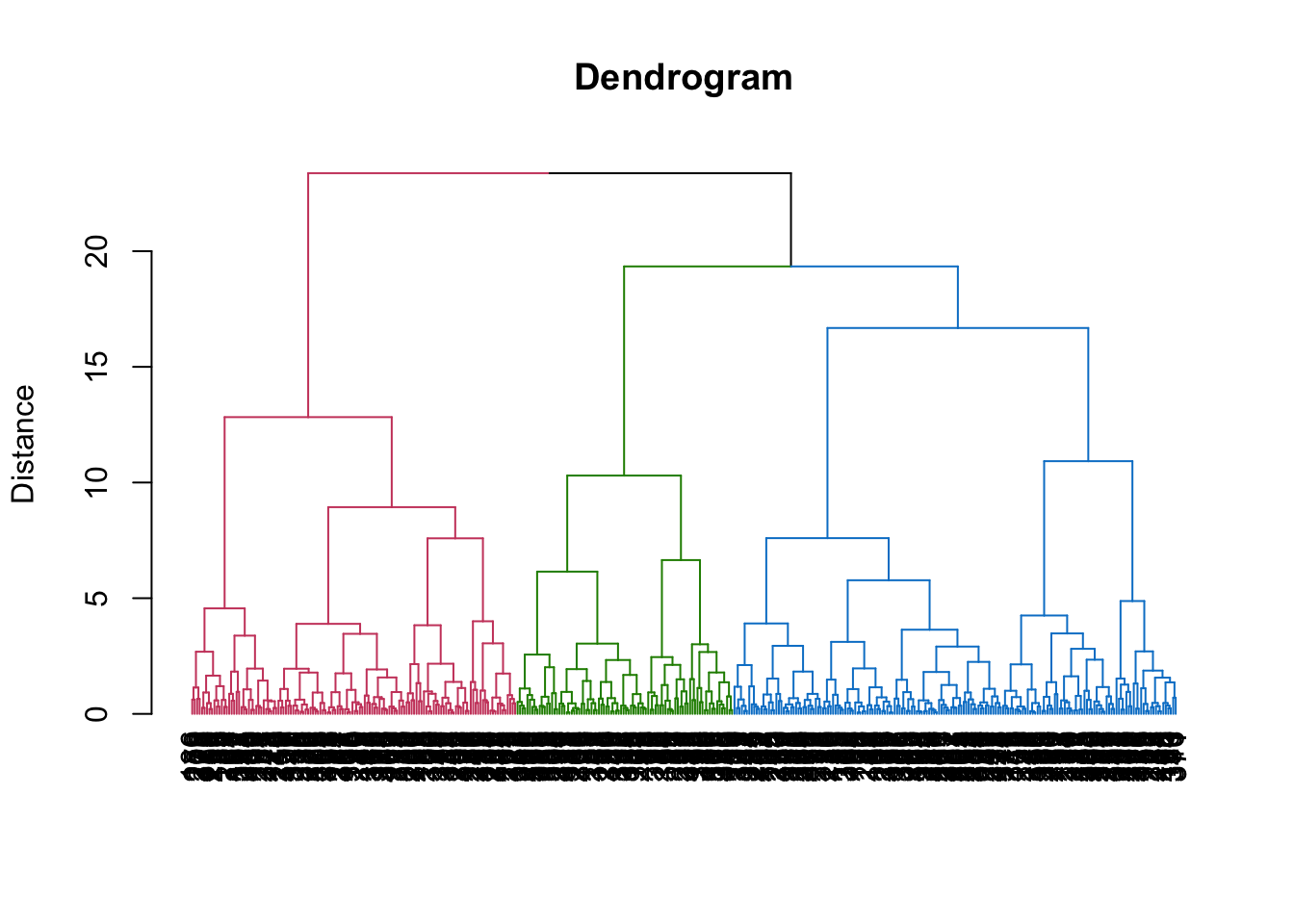
6.2 K-Means
set.seed(42)
EFA_kmeans <- kmeans(EFA_feature , centers = 3)
EFA_kmeans
## K-means clustering with 3 clusters of sizes 137, 144, 119
##
## Cluster means:
## PA1 PA3 PA5
## 1 0.638 -0.477 0.722
## 2 -0.952 -0.453 -0.467
## 3 0.417 1.096 -0.266
##
## Clustering vector:
## [1] 2 1 3 2 1 1 3 2 3 2 2 3 2 1 3 3 1 3 2 2 2 2 1 1 3 3 3 3 3 3 2
## [32] 1 1 3 3 3 1 1 1 1 1 3 2 2 3 3 3 3 3 2 3 3 2 1 2 3 2 3 3 3 1 2
## [63] 2 2 1 2 2 1 1 1 1 2 2 1 1 2 2 1 2 3 3 2 2 2 3 2 2 1 3 2 3 3 2
## [94] 3 1 1 1 2 2 2 2 3 2 2 2 1 3 3 1 3 3 3 2 1 2 2 1 2 2 2 3 2 3 1
## [125] 2 2 2 2 1 2 1 1 3 2 2 1 1 1 1 1 1 1 2 2 1 2 3 3 2 2 1 2 3 1 1
## [156] 2 3 2 1 3 3 1 1 2 3 2 1 1 2 3 1 2 2 3 3 1 1 3 3 1 3 2 1 1 3 1
## [187] 1 2 2 3 1 1 2 2 3 2 2 1 3 1 1 2 3 2 1 1 2 1 2 2 3 1 2 1 1 2 3
## [218] 1 2 1 1 2 1 2 1 2 3 2 1 2 2 1 1 3 3 1 3 1 2 1 2 3 3 2 3 2 3 1
## [249] 2 2 3 2 1 1 3 2 3 2 2 1 1 3 3 2 1 1 2 2 3 2 1 3 1 2 1 1 1 1 1
## [280] 3 3 2 1 1 3 2 2 1 3 2 3 2 2 1 1 2 1 3 3 3 1 2 1 1 2 1 1 3 3 3
## [311] 2 2 2 3 2 1 2 3 1 1 2 1 2 3 2 3 2 2 2 3 1 2 3 3 3 3 2 2 1 2 1
## [342] 1 1 1 3 2 2 3 1 2 3 2 1 2 3 3 3 3 3 1 1 1 2 1 3 3 2 1 1 2 3 1
## [373] 1 3 2 3 2 2 1 3 1 1 3 1 1 3 3 2 1 2 1 3 1 3 3 2 2 1 1 2
##
## Within cluster sum of squares by cluster:
## [1] 203 268 204
## (between_SS / total_SS = 43.6 %)
##
## Available components:
##
## [1] "cluster" "centers" "totss" "withinss"
## [5] "tot.withinss" "betweenss" "size" "iter"
## [9] "ifault"# factor plot
fviz_cluster(EFA_kmeans,
data = EFA_feature) +
theme_bw()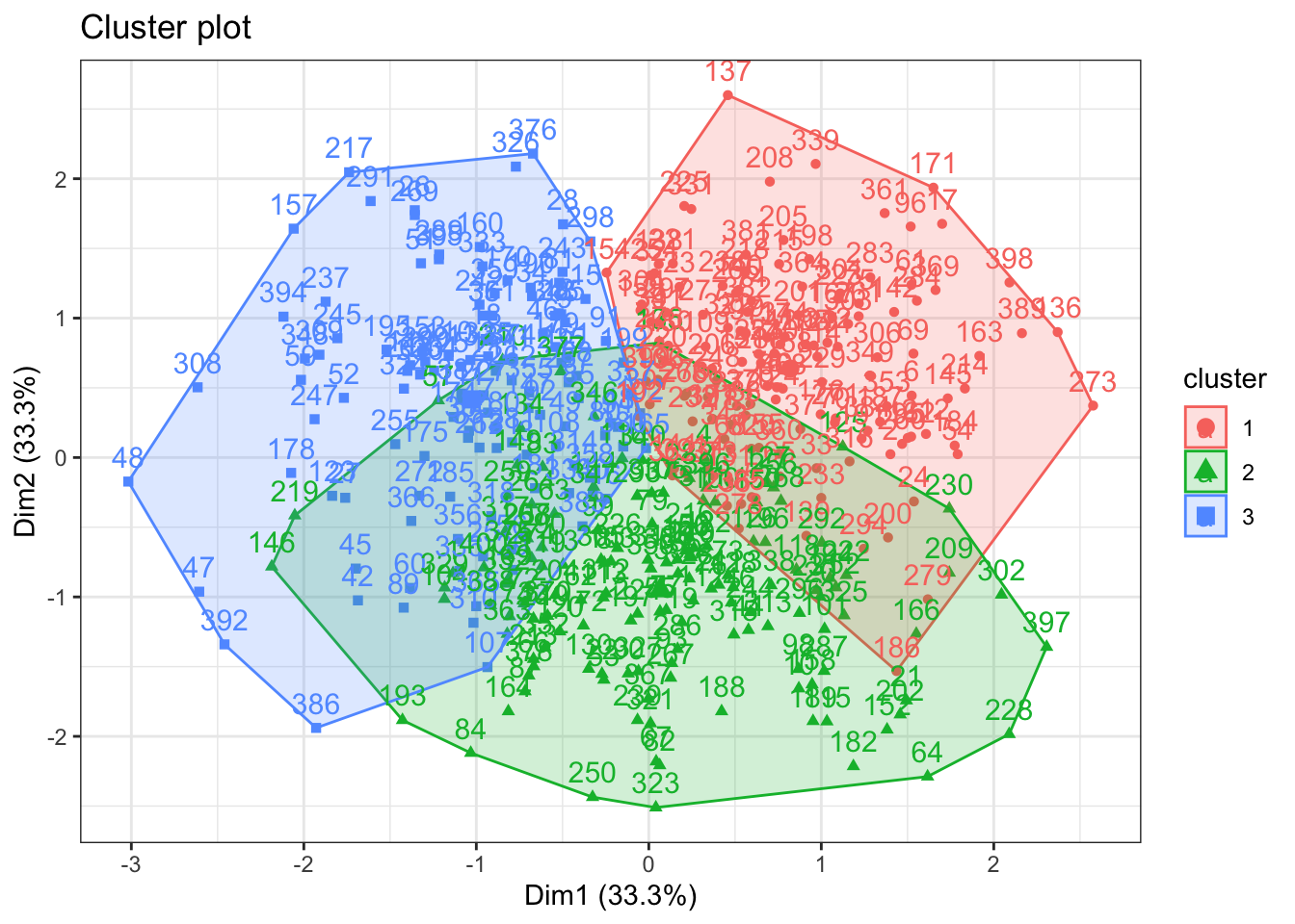
6.3 Interpretation of the results
6.3.1 Heatmap Table
# Average for each cluster with one step
vars_cluster_agg = aggregate(vars_cluster[, 2:31],
          by = list(cluster = EFA_kmeans$cluster),
          FUN = mean)
# reshape
df <- vars_cluster_agg %>%
gather(variable, value, -cluster) # to transfrom from wide to long formatlibrary(gt)
library(scales)
# reshpae, long to wide (cluster )
df_wider = df%>%
dplyr::mutate(cluster = paste0("Cluster", cluster)) %>%
dplyr::mutate(., across(where(is.numeric), round, 2)) %>%
spread(., key=cluster, value =value)
# cluster columns
clusterCols = c("Cluster1", "Cluster2", "Cluster3")
# color
colfunc <- colorRampPalette(c("darkblue", "lightgrey"))
# DT table
DT::datatable(df_wider, options = list(pageLength = 15)) %>%
formatStyle("Cluster1",
backgroundColor = styleEqual(sort(unique(df_wider$Cluster1),
decreasing = TRUE),
colfunc(length(
unique(df_wider$Cluster1)
)))) %>%
formatStyle("Cluster2",
backgroundColor = styleEqual(sort(unique(df_wider$Cluster2),
decreasing = TRUE),
colfunc(length(
unique(df_wider$Cluster2)
)))) %>%
formatStyle("Cluster3",
backgroundColor = styleEqual(sort(unique(df_wider$Cluster3),
decreasing = TRUE),
colfunc(length(
unique(df_wider$Cluster3)
)))) %>%
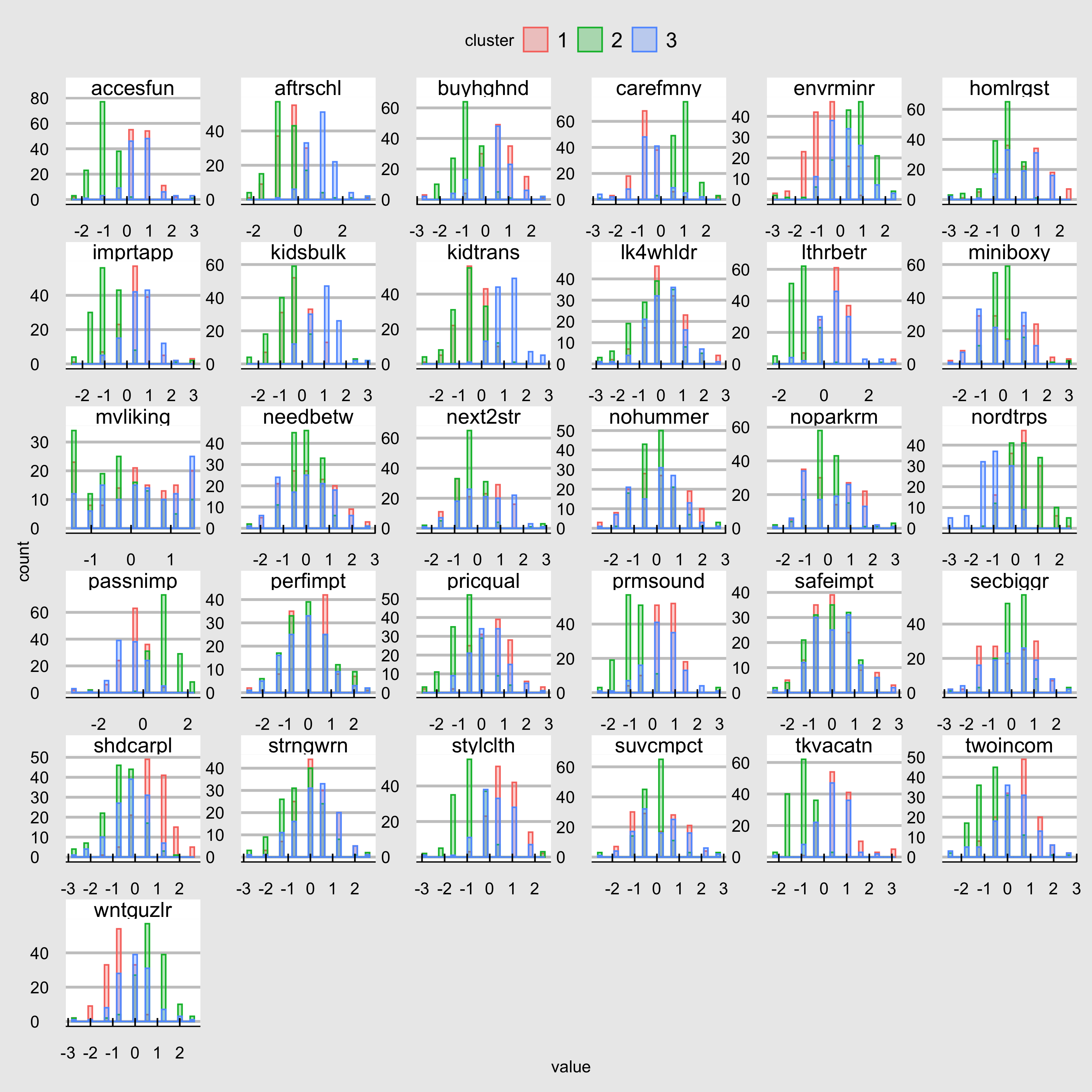
formatStyle(clusterCols, color = "white")6.3.2 Histogram
df = vars_cluster %>%
  gather(variable, value, -cluster)  %>%
  as.data.frame()

# factorize cluster
df$cluster <- factor(df$cluster)

# plot
vars_cluster_hist = ggplot(df, aes(value,
                     fill = cluster,
                     color = cluster)) +
  geom_histogram(alpha = 0.3, position = "identity")  +
  facet_wrap( ~ variable, scales = "free",ncol = 6)  +
  theme_economist_white()

vars_cluster_hist_path = file.path(plotDir, "vars_cluster_hist.png")

ggsave(
  filename = vars_cluster_hist_path,
  plot = vars_cluster_hist,
  width = 3000,
  height = 3000,
  units = "px"
)