Chapter2 Explorative Data Analysis

---

# data 
dataPath = file.path(dataDir, "microvan.csv")
microvan = read.csv(dataPath, sep=";")

# Convert all integer variables into numeric ones for futher work
microvan <- as.data.table(lapply(microvan, as.numeric))

# data description
description = psych::describe(microvan) %>%
  as.data.frame() %>%
  tibble::rownames_to_column(.,var="variable") %>%
   dplyr::select(vars,everything())%>%
  dplyr::rename(., "variable id" = "vars")
 

# columns that need to be formatted
numCols = c("mean",
                    "sd",
                    "median" ,
                    "trimmed",
                    "mad",
                    "min",
                    "max",
                    "skew",
                    "kurtosis",
                    "se")
DT::datatable(
  description,
  rownames = F,
  fillContainer = T,
  options = list(
    pageLength = 10,
    scrollX = TRUE,
    scrollY = TRUE
  )
) %>%
  DT::formatRound(columns = numCols , digits = 1)

2.1 Histogram

microvan_df = microvan[,2:32] %>%
  gather()

microvan_hist =
  ggplot(microvan_df, aes(value)) +
  facet_wrap(~ key, scales = "free",ncol = 6) +
   geom_histogram(alpha = 0.5, position = "identity")  + theme_economist_white() +theme(axis.title.x = element_blank())

microvan_hist_path = file.path(plotDir, "microvan_hist.png")
ggsave(
  filename =microvan_hist_path,
  plot = microvan_hist,
  width = 4000,
  height =4000,
  units = "px"
)

## `stat_bin()` using `bins = 30`. Pick better value with
## `binwidth`.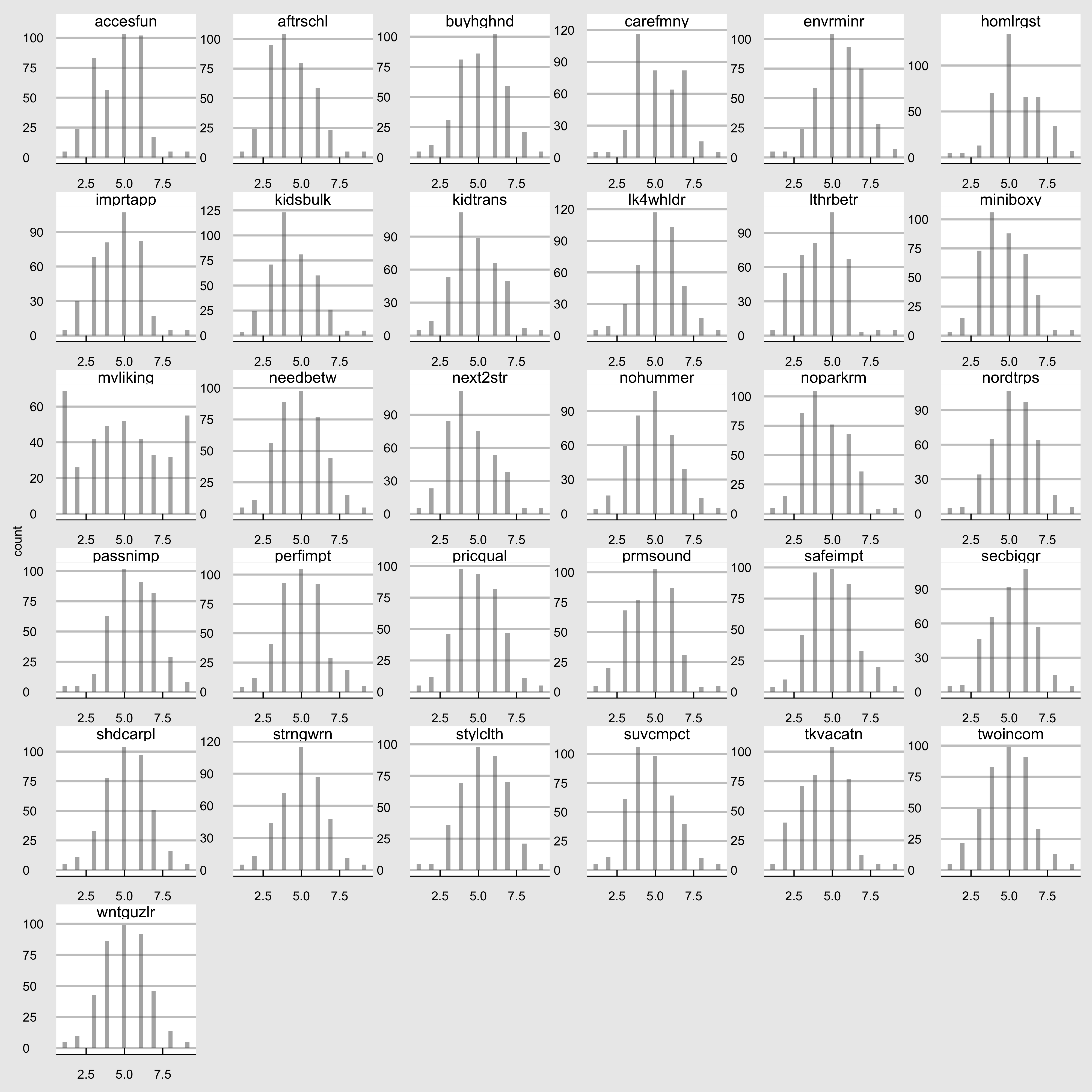

Figure 2.1: Variable 2-32

2.2 Correlation Analysis

2.2.1 Pair-wise Scatter Plot

2.2.2 Correlation Matrix

# plot name
corrPlot = file.path(plotDir, "corrPlot.png")
cor_with_mvliking <- cor(vars)
png(
  filename = corrPlot,
  width = 1500,
  height = 1500
)

corrplot(cor_with_mvliking, 
         method="number", 
         type="upper", 
         order = "hclust", # reorder by the size of the correlation coefficients
         tl.cex = 1.5,     # font size of the variable labels
         tl.col = "black", # color of the variable labels
         tl.srt = 45,      # rotation angle for the variable labels
         number.cex = 1.4    # font size of the coefficients
)
invisible(dev.off())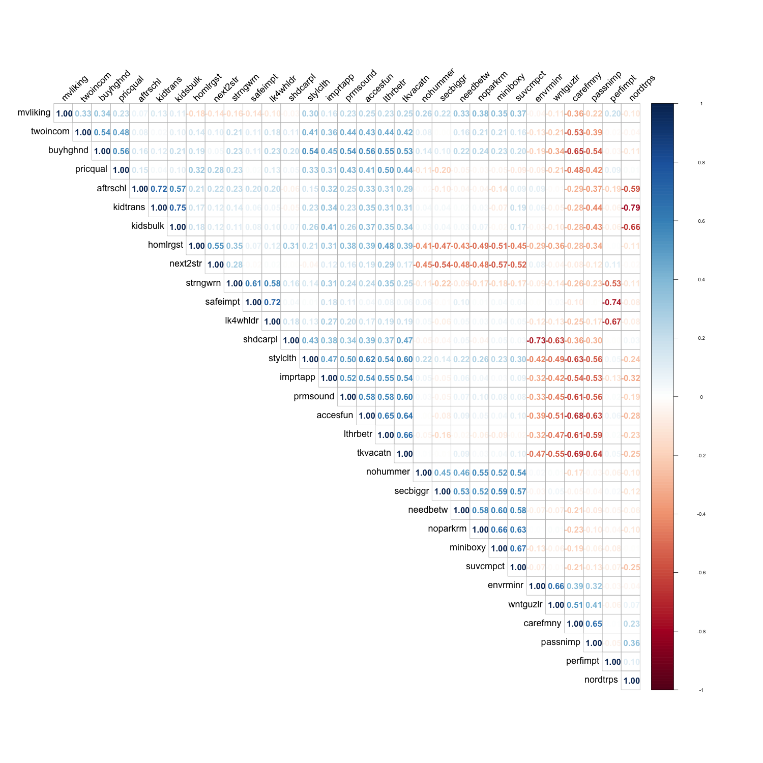

2.2.3 Normality test

options(digits = 3)
df_test= microvan[, 2:32] 
lshap = df_test%>%
  
  summarise_all(.funs = funs(#statistic = shapiro.test(.)$statistic,
    p.value = shapiro.test(.)$p.value)) %>%
  t() %>%
  as.data.frame() %>%
  tibble::rownames_to_column(., var = "variable") %>%
  dplyr::rename(., pvalue = "V1") %>%
  #  data is normal if the p-value is above 0.05
  dplyr::mutate(normality = case_when(pvalue > 0.05 ~ "normal",
                                      pvalue <= 0.05 ~ "not_normal"))

normal_v =  lshap%>%
  filter(normality =="normal") %>%
  pull(variable)
  
shapiro.test(df_test$mvliking)

## 
##  Shapiro-Wilk normality test
## 
## data:  df_test$mvliking
## W = 0.9, p-value = 1e-13